Cool Tool: Hedge Algorithm
The Problem
The idea of the Hedge algorithm is to solve the Expert Advice Problem: Given that we have different experts making a prediction, how do we determine the most accurate prediction or weight them in such a way to get the most accurate prediction?
This post was inspired off of these posts:
Example Problem
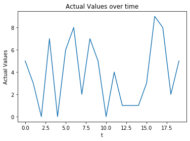
We are going to phrase the following problem as the following: we are going to generate random integers over lets say 20 time periods and call this the actual signal.
actual_values = np.random.randint(0,10,size=[20])
plt.plot(actual_values)
plt.ylabel("Actual Values")
plt.xlabel("t")
plt.title("Actual Values over time")
Now lets say we have n=5 predictors, lets consider having different expert predictions now and consider “creating” an expert by using a function to modify what the actual value is with some random noise with a fixed standard deviation.
def create_expert(std,actual_values):
    return actual_values+np.random.randn(actual_values.size)*std
# Fixed Standard Deviations for each expert
stds = [1,0.1,0.03,0.5,1.3]
expert_predictions = np.array([create_expert(std,actual_values) for std in stds])
plt.title("Actual Value versus the Expert Predictions")
plt.plot(actual_values,linewidth=2,label="Actual Value")
plt.plot(expert_predictions[0],'ko',label="Expert 1")
plt.plot(expert_predictions[1],'bo',label="Expert 2")
plt.plot(expert_predictions[2],'ro',label="Expert 3")
plt.plot(expert_predictions[3],'go',label="Expert 4")
plt.plot(expert_predictions[4],'yo',label="Expert 5")
plt.ylabel("Values")
plt.xlabel("t")
plt.legend(bbox_to_anchor=(1.0, 1.0))
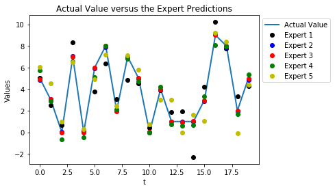
Here is a cross section of the predict values from our experts at a specific time.
expert_predictions[:,0]
array([5.03248168, 4.87141588, 4.9364445 , 5.72195663, 6.04180341])
So how are we supposed to weight the experts correctly to get as close to the actual value as possible? Let’s code an online algorithm for the Hedge Algorithm.
def define_epsilon(n,T,a=1):
    """
    Calculates a factor that is used in determining loss in the hedge algorithm

    Args:
        n (int): number of experts present
        T (int): number of time steps taken
        a (float): value that we can use to scale our epsilon
    Return:
        epsilon (float): the theoretical episilon, but which can be customized by a
    """

    return np.sqrt(np.log(n)/T)*a

class onlineHedge(object):

    def __init__(self,n=10,T=10,a=1):
        self.n = n
        self.T = T
        self.weights = np.ones(n)/n
        self.epsilon = define_epsilon(self.n,self.T,a=a)

    def weight(self,expert_predictions,actual_value):
        """
        Will recalculate the weights on each of the experts based off of the expert predictions and the actual value.
        This can only be done after the actual value is known.

        Args:
            expert_predictions (np.array) (pred.float): np.array with the expert predictions
            actual_values (float): float of the actual value here

        Returns:
            Nothing
        """

        #Calculating losses
        losses = se(expert_predictions,actual_value)

        #Apply weights
        reweighting = np.exp(-self.epsilon*losses)
        self.weights*=reweighting
        self.weights/=np.sum(self.weights)

    def predict(self,expert_predictions):
        """
        Weights the expert predictions into a single prediction based on the weights that have been calculated by the
        hedge algorithm

        Args:
            expert predictions (np.array) (pred.float): np.array with the expert predictions

        Returns:
            a value for prediction based on the inputs of the experts and their respective weights.
        """

        return np.dot(self.weights,expert_predictions)

    def fit_predict(self,expert_predictions,actual_values):
        """
        Will perform weighting at each time step of historical data in order to fit to the data and also perform online
        predictions. Shows the performance of the algorithm and can be used to check performance.

        Args:
            expert_predictions (np.array) (pred.float,time.float): np.array with the expert predictions across time
            actual_values (np.array) (time.float): np.array with the actual value across time.

        Returns:
            (weights (np.array), predictions (np.array))
        """
        weights = []
        predictions = []
        for i in range(len(actual_values)):
            weights.append(hedge.weights.copy())
            predictions.append(hedge.predict(expert_predictions[:,i]))
            hedge.re_weight(expert_predictions[:,i],actual_values[i])

        return (np.array(weights), np.array(predictions))

def se(actual,expected):
    """
    Will return the squared error between the two arguments
    """
    return np.power(actual-expected,2)

def mse(actual,expected):
    """
    Will return the mean squared error between the two arguments
    """
    return np.mean(se(actual,expected))
Characterization of the Loss Weighting Function
hedge = onlineHedge(n=5,T=20)
hedge.epsilon
0.2836756873997224
#Choosing the proper weighting
weights = []
predictions = []

for i in range(20):
    weights.append(hedge.weights.copy())
    predictions.append(hedge.predict(expert_predictions[:,i]))
    hedge.weight(expert_predictions[:,i],actual_values[i])

weights = np.array(weights)
for i in range(5):
    plt.plot(weights[:,i],label='{}'.format(i+1))
plt.title("Weights on Experts vs Time (t)")
plt.ylabel("Weights")
plt.xlabel("t")
plt.legend(bbox_to_anchor=(1.0, 1.0))
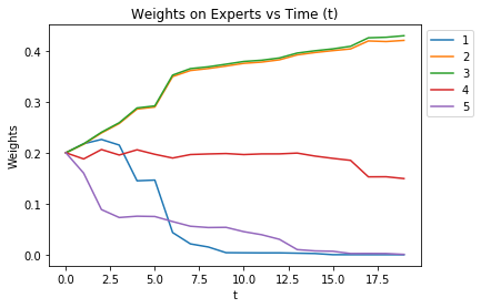
We see that over time, the experts the smallest standard deviations in terms of the errors, or the most accurate, will get the highest weights.
plt.figure()
plt.title("Predicted Ensemble Methods")
plt.plot(hedge.predict(expert_predictions),label="Optimal Hedge Weighting")
plt.plot(predictions,label="Hedge Weighting")
plt.plot(np.mean(expert_predictions,axis=0),label="Average")
plt.plot(actual_values,label="Actual")
plt.ylabel("Actual Value")
plt.xlabel("t")
plt.legend(bbox_to_anchor=(1.0, 1.0))
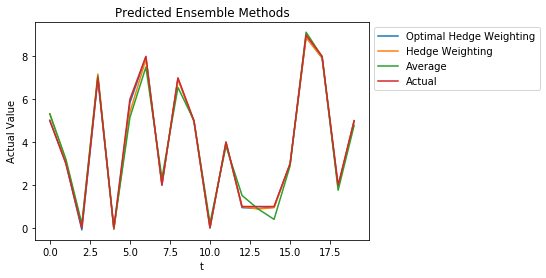
We can also see that the Hedge Weighting provides a much more consistent and accurate estimate for the actual value than taking the average! (The optimal hedge weighting is the hedge weights at the end of training, the hedge weighting represents the online hedge algorithm’s weights that are update as time passes).
Error Analysis
We are first going to calculate the MSE from the actual values and a weighted average of the expert’s values. The first weights we are going to use are the best weights after training for the entire period.
mse(hedge.predict(expert_predictions),actual_values)
0.0039610981057562195
Now we are going to see the MSE from the online Hedge Algorithm as it changes weights and updates over time.
mse(predictions,actual_values)
0.030779479858401525
We are now also going to include the MSE from just simply averaging the predictions from the “experts”.
mse(actual_values,np.mean(expert_predictions,axis=0))
0.11710251002013569
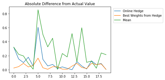
We notice that if we use the predictions from the optimal weights we get a very low MSE, almost an order of magnitude better than if we were to use the online algorithm. The improvement between the online algorithm and just taking the average of the experts is almost 3x as good which means instead of taking the mean of predictions in this case to estimate the actual value, we should try to use the online hedge algorithm instead. If we look at absolute difference between the actual value and the predictions from the different methods over time we get:
plt.title("Absolute Difference from Actual Value")
plt.plot(abs(predictions-actual_values),label="Online Hedge")
plt.plot(abs(hedge.predict(expert_predictions)-actual_values),label="Best Weights from Hedge")
plt.plot(abs(np.mean(expert_predictions,axis=0)-actual_values),label="Mean")

plt.legend(bbox_to_anchor=(1.53, 1.0))
Applications and additional discussion
This hedge algorithm should be used for determining which portfolio strategy is best as well as trying to perform accurate predictions for values based on analysts or researchers. In general it would be really interesting to see this applied to analyst predictions or in essemble methods since this is very basically like Adaboosting in decision Trees. A really great explanation of Adaboosting is linked here.